![You are currently viewing How to Find, Highlight & Remove Duplicates in Google Sheets [Step-by-Step]](https://www.dimaservices.agency/wp-content/uploads/2024/04/e7cd3f82-cab9-4017-b019-ee3fc550e0b5.png)
Duplicate data is the bane of spreadsheet solutions, especially at scale. Given the volume and variety of data now entered by teams, it’s possible that duplicate data in tools like Google Sheets may be relevant and necessary, or it could be a frustrating distraction from the primary purpose of spreadsheet efforts.
The potential problem raises a good question: How do you highlight duplicates in Google Sheets?
I’ve got you covered with a step-by-step look at how to highlight duplicates in Google Sheets and find duplicates in Google Sheets, complete with images to ensure you’re on the right track when it comes to de-duplicating your data.
Table of Contents
- How to Find Duplicates in Google Sheets
- Highlighting Duplicate Data in Google Sheets
- Step-by-Step: How to Highlight Duplicates in Google Sheets (With Pictures)
- How to Highlight Duplicates in Multiple Rows and Columns
- How to Remove Duplicates in Google Sheets
How to Find Duplicates in Google Sheets
Google Sheets is a free, cloud-based alternative to proprietary spreadsheet programs and — no surprise, since it’s Google we’re dealing with — offers a host of great features to help streamline data entry, formatting, and calculations.
There are two ways to remove duplicates in Google Sheets: conditional formatting and the UNIQUE function. I’ll go over both below, but, before you start following along, I have two things to note:
- You can run multiple conditional formatting rules at a time, so you don’t need to delete any to run your conditional formatting rule to delete duplicates.
- You won’t get an accurate duplicate count if you have any extra characters or spaces in your data, so you need to make sure your set is clean. Even an accidental extra space will count it as a separate data point.
Let’s dive into how you can highlight and remove duplicates in Google Sheets.
Highlighting Duplicate Data in Google Sheets
Google Sheets has all the familiar functions: File, Edit, View, Format, Data, Tools, etc., and makes it easy to quickly enter your data, add formulas for calculations, and discover key relationships.
While other spreadsheet tools, such as Excel, have built-in conditional formatting tools to pinpoint duplicate data in your sheet, Google’s solution requires a little more manual effort.
So how do you automatically highlight duplicates in Google Sheets? While there’s no built-in tool for this purpose, you can leverage some built-in functions to highlight duplicate data.
Step-by-Step: How to Highlight Duplicates in Google Sheets (With Pictures)
Here’s a step-by-step guide to highlighting duplicates in Google Sheets:
Step 1: Open your spreadsheet.
Step 2: Highlight the data you want to check.
Step 3: Under “Format”, select “Conditional Formatting.”
Step 4: Select “Custom formula is.”
Step 5: Enter the custom duplicate checking formula.
Step 6: Click “Done” to see the results.
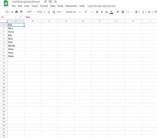
Step 1: Open your spreadsheet.
First, head to Google Sheets and open the spreadsheet you want to check for duplicate data.
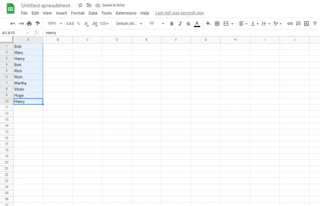
Step 2: Highlight the data you want to check.
Next, drag your cursor over the data you want to check to highlight it.
Step 3: Under “Format”, select “Conditional Formatting.”
Now, head to “Format” in the top menu row and select “Conditional Formatting.” You should then see a popup window titled “Conditional format rules.”
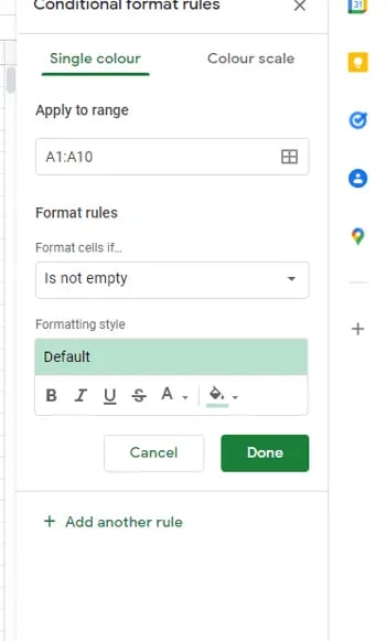
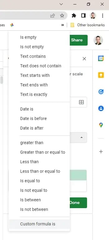
Step 4: Select “Custom formula is.”
Next, you need to create a custom formula. Click the down arrow underneath “Format cells if,” and select “Custom formula is” from the dropdown menu. It’s the last option to choose from, so you can scroll right to the end.
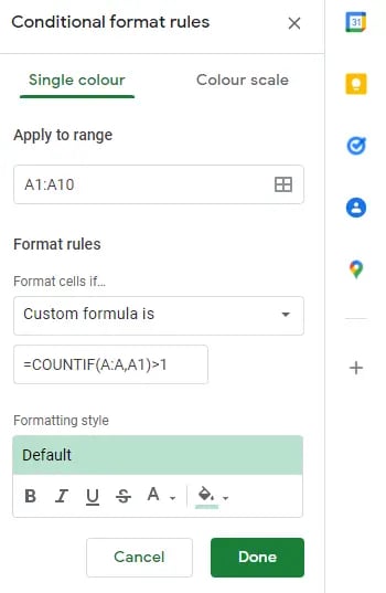
Step 5: Enter the custom duplicate checking formula.
To search for duplicate data, we need to enter the custom duplicate checking formula, which for our column of data (A) looks like this:
=COUNTIF(A:A,A1)>1
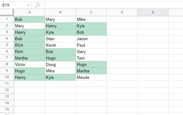
The formula searches for any text string that appears more than once in a data set. The default highlight color is green, but you can change it by clicking on the paint can icon in the “Formatting style” menu.
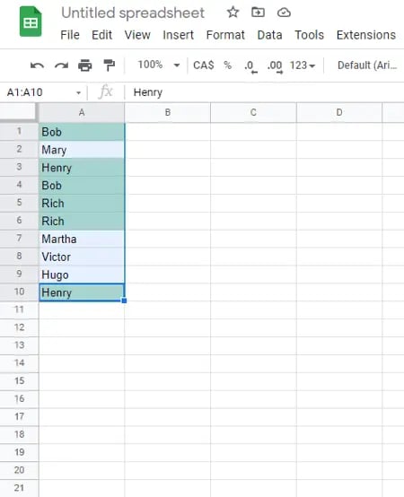
Step 6: Click “Done” to see the results.
And voilà — we’ve highlighted the duplicate data in Google Sheets.
How to Highlight Duplicates in Multiple Rows and Columns
You can also highlight duplicates in multiple rows and columns if you have a larger data set. The process starts the same as above, but you enter an expanded data range in the Conditional format rules menu to account for all the cells you want to compare.
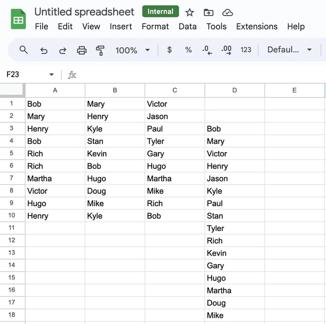
I’ll use the same example above as a starting point, but I’ll add a few more names so we use a formula to search across three columns: A, B, and C, and also across rows 1-10.
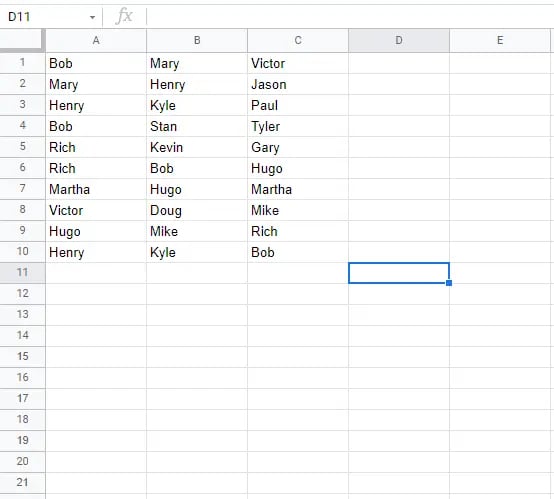
To start, repeat steps two – four from above, but enter the following equation during step 5:
=COUNTIF($A$2:G,Indirect(Address(Row(),Column(),)))>1
This will highlight all duplicates across all three columns and all ten rows, making it easy to spot data doppelgangers:
Find and Highlight Duplicates in Google Sheets With the Unique Function
Another way to find duplicates in Sheets is to use the UNIQUE function, which looks for the unique values in your designated range and produces a duplicate-free list. Here’s the formula:
=UNIQUE(RANGE)
Note: This formula can only identify duplicates in a single column.
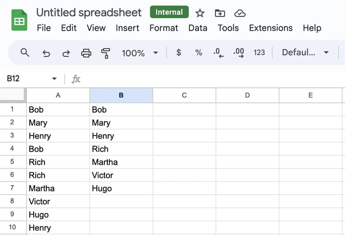
There’s only one step to this method, which is entering your formula into an empty cell. Continuing with the same data set from above, I entered =UNIQUE(A1:A10). The image below is my duplicate-free list (on the left).
To use the UNIQUE function to find duplicates in multiple columns and rows, use this formula:
=UNIQUE(TOCOL(RANGE))
A drawback to using the UNIQUE function to find duplicates in Google Sheets is that it spits out a separate duplicate-free list instead of highlighting and deleting them. It creates an added step since you’ll have to manually remove duplicates with your new list as a reference, so I recommend this method for those with a smaller data set who don’t mind a few manual updates.
Alternatively, this method is an excellent option for producing a cleaned list to start fresh.
How to Remove Duplicates in Google Sheets
In addition to highlighting duplicates, you can also use Google Sheets to delete duplicates with the Data Cleanup feature. Below, I’ll show you how.
Step 1: Select any cell.
Step 2: Navigate to the header toolback, select “Data,” then “Data cleanup,” then “Remove duplicates.”
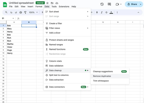
Step 3: In the popup window, select the columns you want to delete duplicate data from, then select “Remove duplicates.
Note: If you have a sheet header, make sure to select “Data has a header row” so it’s not included in the duplicate search.
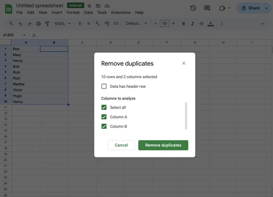
All duplicates are now gone!
Dealing With Duplicates in Duplicates in Google Sheets
Can you highlight duplicates in Google Sheets? Absolutely. While the process takes more effort than some other spreadsheet solutions, it’s easy to replicate once you’ve done it once or twice, and once you’re comfortable with the process you can scale up to find duplicates across rows, columns, and even much larger data sets.
![]()